Over the last couple of weeks, we have mainly focused on wrapping up loose ends, with filling out data that we’d already got equations for, fixing some error parts, and some other little bits here and there. But the end is in sight! Report writing is now well underway, hoping to get it done with some days to spare, for reading over and checking everything. A slight spanner in the works has been thrown in that we are actually not expected to have a theory section and instead it should be integrated into other sections of the report. After having thought about it for a little while, Harry and I discussed it and came to the conclusion that just continuing what we were doing was best and then copy pasting bits and bobs from the theory and putting it in other sections instead once everything was finished was what would work best. This would allow us all to continue working on our separate sections without getting in each other’s way. This does mean that some parts may need rewording at the end, but this is again part of the reason we hope to finish with enough time before the deadline.
We also have created a presentation with some plots and results and a summary of our project to present to our peers at the end of week 18, which took up a lot of our time. It was a good opportunity to prepare for the PLACE mini-conference, which takes place later this year.
Monte Carlo method
Other than finishing off loose ends, another aspect that we have been focused on, but particularly Harry is using the Monte Carlo method to get our final number of planets that fit within these parameters and their error. This method fits Gaussian’s over all parameters within two standard deviations and after running it 100 times, an average is found and it gives a realistic estimate with errors for the amount of planets that fit into our parameter limitations, accounting for errors.
The results found for different limits of our parameters can be seen here:
We have spent the last few weeks writing the scientific report that explains the background and methodology of our investigation in more detail and further analyses and discusses the data above. If you are interested in reading it, it will be published in this Summer’s edition of NLUAstro, with the other PHYS 369 Group Projects from this year, so please keep an eye out for it.
This post is a short summary of the last few weeks’ work.
Habitable Zone Research
Owen did some research into calculating the habitable zone for exoplanets. He found a pair of very simple equations corresponding to the inner and outer edge of the habitable zone:
The inner Edge of the HZ (r_i) is the distance where runaway greenhouse conditions vaporize the whole water reservoir and, as a second effect, induce the photodissociation of water vapor and the loss of hydrogen to space. The outer edge of the HZ (r_o) is the distance from the star where a maximum greenhouse effect fails to keep the surface of the planet above the freezing point, or the distance from the star where CO2 starts condensing.
The article Owen found these equations on backs using the Stellar Flux over equilibrium temperature which cancels any dependence on albedo. This makes determining values for Stellar Flux’s easier as albedo differs only slightly in every spectral type of star. This article came to the conclusion of using 0.53W/m^2 and 1.1W/m^2 for the outer and inner stellar flux’s, respectively, by using the bolometric correction. These values were clarified in [Kasting et al., 1993, cited below; Whitmire et al., 1996].
We wanted to create our own formula, with different assumptions, to compare with equations Owen had found. Amaia did some research into this and found an equation that we could manipulate:
We rearranged this equation to make the orbital radius D the subject and then subbed in temperature limits to find the inner and outer limits of the habitable zone radius. For our temperature limits we used:
647K – critical temperature of water
273K – freezing point of water
When creating our own formula for the habitable zone, we made a few assumptions on the way. We started off by assuming the planets are black bodies, meaning the albedo a is 0 and emissivity ε is 1.We set the ratio of the area of the planet that absorbs power Aabs and the area of the planet that radiates power Arad to ½, which assumes a slow-rotating planet and makes sense as only about half of the planet will be facing the star at a time. We have assumed a circular orbit as we use a sphere radius of D. We have also assumed no greenhouse effect and an even temperature around the planet, which is not the case but is taken as an average.
Determining Parameters to Define our ‘Habitable Planet’
Amaia and Harry selected which parameters we would use as our definition of a habitable planet and have determined value ranges for each parameter.
Max Gravity: (3-4)g
Minimum mass: 0.3 Earth Masses
Stellar star classification: F, G, K
Temperatures associated with these spectral types: F(6000K-7600K), G(5000K-6000K), K(3500K-5000K)
Habitable Zone: We will use the equation Owen found and the one we create ourselves
Planet Density: >2000kg/m^3 (anything less is probably a gaseous planet)
Kepler’s Law
Harry found that Kepler’s law does hold for our dataset (with very circular orbits of single-star systems). Nevertheless, we couldn’t just decide to dismiss all eccentric orbits as this would eliminate a huge amount of our data.
Amaia suggested to use the circular, single star orbits to prove that Kepler’s law fits the dataset, and then use the specific relationship for the whole dataset to fill in the values. We spoke to David about this issue, and he suggested that orbital periods longer than the time we’ve been observing exoplanets for can skew the data. This might be contributing to the issue too. The periods longer than we’ve been studying exoplanets will have large errors and therefore give large errors. David also pointed out that Kepler’s Law should use the average distance not just “a”. The distance measured as “a” for some planets may simply be the detected distance, not an actual calculation of “a”. This is more to do with the way the database is written. If there is an accurate period given, it should always give you the average distance “a”. So, we just used Kepler’s law to fill in the gaps and propagated the errors.
Applying Kepler’s law to our dataset proved to be difficult and so Davids feedback was to not bother checking specifics with weird periods and eccentricities. We Just assumed Kepler’s law works for all because they are all within the same order of magnitude, so this is a reasonable assumption for astrophysics. Plus, the number of stars in the system doesn’t have much of an effect. In the end we concluded that it’s hard to prove that Kepler’s law holds for the data set we have, but we can assume it does for every star because it’s a geometric law. Also applies to semi major axis of course.
Calculating errors for our data
Amaia has calculated all the errors with a lengthy code that contains a lot of separate functions. Amaia found the difference between actual radius and calculated radius (and for mass) for the ones we have both for. Using bins instead of plotting all of them, she found the average deviation for the values in that bin. Too many small bins lead to empty bins, so she widened them enough that it worked. She added a linear relationship on either end of the mass-radius ranges rather than extrapolating outside the range to fit higher and lower values, because extrapolating didn’t return sensible values. Extrapolating for the other values were however successful.
Multiple Star Systems
In our dataset, we realise that a portion of these exoplanets orbit star systems of more than one star. Owen did some research into multiple star systems to see whether this would affect our results.
When a planet orbits a multiple star system, it can orbit the stars in several ways. For example, in a binary star system, the planet can either orbit one star (S-type orbit) or orbit both stars (P-type orbit). This qualitive information is not available in our dataset. So before proceeding into further research, we knew that this research wouldn’t be changing our results but would be good to include in our discussion section for the report.
Multiple-star systems can perturb a planet’s orbit, precluding any chance for life as we know it to survive. But even for planets in stable orbits, these stars can produce habitable zones that change dramatically as the stars move around each other. Habitable planets can dip out of the HZ for a small amount of time, and the resilience of the planets habitability strongly depends on its climate inertia. Combining orbital dynamics with simple climate models we demonstrate that the size of circumstellar habitable zones depends on a planet’s climate inertia. The higher a climate’s resilience to variations in the incident light, the higher the chances for planets to remain in a habitable state. In systems like α Centauri, a low climate inertia shrinks the habitable zone by 50%
Having thoroughly researched what defines a “habitable planet,” we came to a decision on what exactly our research question would be. The end goal of our project will be to find an estimation of f_sp from the CETI equation. This equation aims to calculate the number of intelligent alien civilisations currently in the galaxy, with whom we could communicate. According to the equation, the number of CETI (Communicating Extra-Terrestrial Intelligent civilisations) depends on a number of factors, including f_sp, the fraction of stars in the galaxy which host at least one suitable planet, in a habitable zone, which could support life, out of all the stars in the Galaxy which are older than 5Gy.
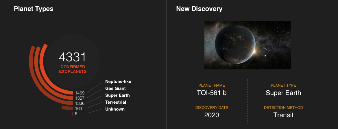
To find an estimate for this, we need to analyse as much data about exoplanets in our galaxy as we can, and filter it according to our definitions of “suitable planet, in a habitable zone” and we will achieve this using data from the NASA Exoplanet Archive. The archive includes a catalogue of data for exoplanets which have been discovered and about which there is published research, among a number of other resources. This particular database contains a wealth of information both about exoplanets and the stars they orbit, including but definitely not limited to masses, radii and orbit periods of planets and temperatures and spectral types for their host stars. This database has specifically been designed to be easy for researchers to work with, with so many characteristics all in one place.
(The exoplanet database contains a lot of columns, many of which are not relevant to our investigation.)
You might think, therefore, that it would be relatively easy to then add some simple filters based on the constraints we researched in the previous week, count how many planets fit all of our criteria for “habitable” and then calculate a value for f_sp (this being our ultimate project aim).
If only it were that simple…
Due to the use of a variety of methods to detect the planets, not every planet has an entry for every variable, leading to “holes” in the data. This is where the bulk of our scientific work has been targeted so far, and it is likely to be that way for most of the length of the project. Some variables have established relationships to each other, based on well-understood physical characteristics. For example, Kepler’s 3rd Law directly relates the semi-major axis of an elliptical orbit with the orbital period and knowing one of these variables should allow the other to be found with relative ease. Others are a little more complex.
One of the criteria we identified as necessary for humans to survive is to have a surface gravity strength within the correct range. The surface gravity of a planet depends on its mass and radius according to Newton’s Law of Universal Gravitation, butnot every exoplanet in the table has entries for both mass and radius. Since the density of an exoplanet (i.e. the relationship between mass and radius) is dependent on its material composition, which is as yet unknown for many of these, it is not possible to directly infer one from the other. Our solution was to derive a relationship between mass and radius for all those that had entries for both, and then apply this relationship to the rest of the planets to fill in the gaps, making it then possible to estimate the surface gravity for every planet.
Harry and Amaia have been spending weeks 3 and 4 doing exactly that. Harry found a linear log-log relationship between the planets’ masses and radii, and used it to find the missing values for the other exoplanets. He then used these values to estimate the surface gravity of these planets. The plot for the known masses and radii (from which the relationship was derived) can be seen below. Although the actual distribution of points looks a bit more like a kingfisher than a straight line, the simple linear relationship is a good enough approximation to first order.
The final relationship is Log10(R) = 0.395(Log10(M)) + 0.0943
When it came to calculating the errors in these new values though, they had some initial difficulty. Originally, the errors were calculated in such a way that they were not independent from one another, and changed depending on whether the missing radii or masses were filled in first. This was clearly not ideal. Then, the plan had been to calculate the errors individually for each exoplanet, but this idea led to complications with the code, and was overly detailed. After some consultation with David, Amaia is now working on code that will assign mass and radius errors based on the range in which the values lie. The hope is that once the code that is being developed has been used successfully on one pair of variables, it could be repurposed relatively easily for other combinations. This has been an excellent example of how projects like this are not always smooth sailing, but still always contain opportunities to learn.
Our plan for thenext week is to fix the errors in the newly calculated mass and radius values, which allows us to accurately calculate the errors in the gravitational field strength estimates. We also hope to use Kepler’s 3rd Law to begin filling in missing values for orbital radius, which can be used to determine whether or not a planet orbits in its host star’s habitable zone.
During the past couple of weeks, we have been working as a group, researching parameters that might be appropriate to determine a planet as habitable, and their boundaries according to past research.
Mass/Gravity
Our data lead Harry did some research into boundaries of what gravity humans could withstand. Harry found an article claiming that humans could withstand a gravity of up to 3-4 times the strength of Earth’s. It is conclusive that these humans would have to have had considerable training to increase their muscle mass and cardiovascular fitness to endure this new strength of gravity. A test was carried out with participant Hafthor Bjornsson(aka The Mountain), former world’s strongest man) where he was put under the simulated conditions of 5 times the Earth’s gravity. He had passed the test but not everyone has the freak genetics of this elite athlete. For most humans, 5g causes near impossible locomotive motion due to the stress on the bones. We concluded that habitable exo-planets have an upper bound value of 4g.
Searching for the lower bound proved to be more difficult as most articles only discuss 0g. However, this could be an interesting discussion point as our journey to exoplanets may have to be on spaceships, where we would be under 0g. The effects of prolonged periods on a spaceship with 0g would weaken our bones and muscles, which would be bad news if we were migrating to an exo-planet with gravity stronger than Earths. Further studies shows that bones lose about 1% density per month (elderly Earth-bound humans lose about 1.5% per year) when in 0g environments. Without any exercise, muscle mass could fall by 20% after 6-11 days.
With further research, an article was found stating they found a critical mass of 0.3 Earth Masses as the lower bound for planetary masses life can exist. This is as a result of deteriorating tectonic activity needed for life to survive.
Atmospheres
Amaia, our group coordinator, did the research for atmospheres of habitable exo-planets. One important property of atmospheres that was explored was pressure. Pressure is significant as it affects the boiling point of water, which is essential for life. Amaia came across a significant term called the Armstrong Limit. This is the pressure at which atmosphere pressure is sufficient for water to boil at the temperature of the human body. This leads to no life. This led to the conclusion that the lower limit of habitable pressure would be around 75kPa.
The upper limit of pressure was interestingly found through deep sea diving. It is confirmed that with a pressure below 4 bar, the body can function relatively normally but for no change in functioning, the limit is 2 bar.
Amaia also investigated the chemical composition of exo-planets with signs of life and explored deeply into their biosignatures. These compounds consisted of methane, oxygen, nitrous oxide and ammonia (caused by bacteria). We concluded that signs of some of these biosignatures were more signs for already existing life and that discovering a planet with these signatures would be groundbreaking, and therefore an unrealistic expectation. However, properties that are still essential to look for ozone-to protect us from solar flares and harmful UV rays, and water, in order to sustain life.
Spectral Types of Stars
Owen, the communications lead, researched which spectral types of stars would be the best candidates for habitable exo-planets to be orbiting. The types of stars were narrowed down to F, G, and K type stars. This because star types higher up on the spectrum have short life spans on the main sequence. This forbids the evolution of life and prohibits the sufficient time to develop complex life on land like trees and ither types of vegetation.
On the opposite extreme, stars with less than half of the Sun’s mass are more likely to tidally lock planets that are orbiting close enough to have liquid water on their surface too quickly, before life can develop. Tidally locking (or synchronous rotation of the star and planet) may eventually cause the destruction of a life-sustaining atmosphere through condensation on the cold, perpetually dark side of the planet. Moreover, most M-type red dwarf stars would tend to sterilize life on a close-orbiting Earth-type planet regularly with large stellar flares.
Therefore, NASA’s proposed Kepler Mission will search for habitable planets at nearby main sequence stars that are less massive than spectral type A but more massive than type M –dwarf stars of types F, G, and K. However, since low-mass M-and K-type stars so numerous, some astronomers and planetary scientists are continuing to model low-mass stars and possible planetary environments that may be potentially suitable for Earth-type plant and animal life, as well as for microbes.